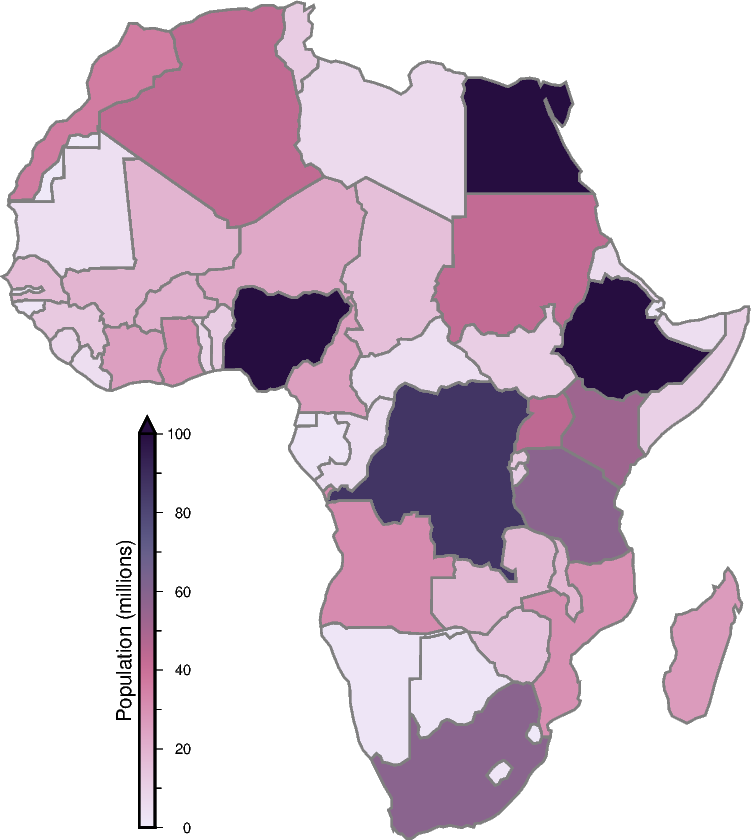
Choropleth map

The pygmt.Figure.plot method allows us to plot geographical data such as polygons which are stored in a geopandas.GeoDataFrame object. Use geopandas.read_file to load data from any supported OGR format such as a shapefile (.shp), GeoJSON (.geojson), geopackage (.gpkg), etc. You can also use a full URL pointing to your desired data source. Then, pass the geopandas.GeoDataFrame as an argument to the data parameter of pygmt.Figure.plot, and style the geometry using the pen parameter. To fill the polygons based on a corresponding column you need to set fill="+z" as well as select the appropriate column using the aspatial parameter as shown in the example below.

import geopandas as gpd
import pygmt

provider = "https://naciscdn.org/naturalearth"
world = gpd.read_file(f"{provider}/110m/cultural/ne_110m_admin_0_countries.zip")

# The dataset contains different attributes, here we focus on the population within
# the different countries (column "POP_EST") for the continent "Africa".
world["POP_EST"] *= 1e-6
africa = world[world["CONTINENT"] == "Africa"].copy()

fig = pygmt.Figure()
fig.basemap(region=[-19.5, 53, -37.5, 38], projection="M10c", frame="+n")

# First, we define the colormap to fill the polygons based on the "POP_EST" column.
pygmt.makecpt(cmap="acton", series=(0, 100), reverse=True)

# Next, we plot the polygons and fill them using the defined colormap. The target column
# is defined by the aspatial parameter.
fig.plot(data=africa, pen="0.8p,gray50", fill="+z", cmap=True, aspatial="Z=POP_EST")

# Add colorbar legend.
fig.colorbar(frame="x+lPopulation (millions)", position="jML+o2c/-2.5c+w5c+ef0.2c+ml")

fig.show()